Quality Assessment of Digital Elevation Models in a Treeless High-Mountainous Landscape
A Case Study from Mount Aragats, Armenia
Abstract Global Digital Elevation Models (DEMs) are widely employed in geoarchaeology. Usually, their adequacy for particular landscapes is not tested. We assessed 30m-resolution-DEMs (ASTER, SRTM, ALOS, EU-DEM, NASADEM, NEXTMap) with local precision datasets. Our results reveal considerable differences (ASTER unsuitable for the region, NEXTMap and EU-DEM fit most closely to our reference model). This outcome does not necessarily apply to all similar regions. It rather stresses the need for a check of DEMs’ quality in any given study area, and it encourages the use of detailed topographic visualisations of DEMs in absence of suitable reference data.
Keywords 30m resolution DEMs. Comparison. Evaluation. RMSE. Spatial analysis. GIS. Landscape archaeology.
1 Introduction1
1 We thank Prof. Dr. Alessandra Gilibert and Ca’ Foscari University of Venice for purchasing the NEXTMap dataset used in this study. We are also grateful to our colleagues from Yerevan – Dr. Arsen Bobokhyan for helping to organize the fieldwork, Dr. Smbat Davtyan for information about topographic measurements and Dr. Shahen Shahinyan for providing us with detailed information about his GPS measurements and the Armenian quasi-geoid. Furthermore, Prof. Dr. Alessandra Gilibert, Michael Rummel, M.A., Stefan Biernath, Ausgr.-Ing. M.Sc., and two anonymous reviewers read the manuscript and provided comments that helped to improve it, which we greatly appreciate. We also extend our thanks to Emma Castle, B.A., for generously proofreading and correcting the final version.
Digital elevation models (DEMs) as approximate virtual representations of terrain have a wide range of applications in archaeology – for visualizations, spatial analysis, predictive modelling etc. (cf. Conolly, Lake 2006; Gillings, Hacıgüzeller, Lock 2020; Siart, Forbriger, Bubenzer 2018 for an overview). Given different understandings of ‘terrain’, terminological distinctions are called for. Currently, DEM is one of three terms used to describe representations of terrain surfaces through sets of heights. The other two terms, with which DEM occasionally is confused and should therefore be delimited from, are a Digital Surface Model (DSM) and a Digital Terrain Model (DTM). While DSM generally designates surfaces that include trees, buildings, and other above-ground objects, the distinction between DTM and DEM is not universally agreed on. DTM and DEM are sometimes used as synonyms designating bare ground surface devoid of natural or human-made above-ground objects. Other times, DTM is the general term for all elevation models and DEM reserved for bare ground surface, or vice versa (Zhou 2017 as opposed to Hirt 2014). In the past, a number of global models were named and distributed as DEMs, although they correspond to DSMs in the terminology prevailing today. For the purposes of this study, we use the DEM term in its general sense – as any digital terrain model with elevation information. In our study area, the treeless and unbuilt character of the landscape means that the terrain has, in most cases, only a single surface which corresponds to the ground level.
In recent years, the increased availability of drones and the advances in multi-image photogrammetry have simplified the creation of detailed DEMs. Elevation models based on low-altitude aerial imagery are thus rapidly becoming a standard practice for smaller sites. For large sites and for regional surveys the DEMs based on LIDAR-data (Light detection and ranging) would be optimal, yet until this data becomes widely available, DEMs obtained with satellite remote sensing methods continue to be the preferred choice. Their continental or global coverage and their availability at (mostly) no cost outweigh the disadvantage of their lower resolution. Indeed, for some applications on regional scale the lower resolution is not even a disadvantage, but rather a desirable necessity. Moreover, the generation of DEMs from satellite data is a dynamic field and in recent years high-resolution datasets with 10m, 5m and even 1m resolution became commercially available for selected areas.2 It can be reasonably expected that in the near future high-precision satellite-derived DEM datasets will reach global coverage and gradually also become available for academic research.
All the current advantages have led us to consider global or continental DEMs for our studies in the Armenian high mountains. Additionally, the treeless character of the studied terrain, which effectively eliminates the danger of vegetation bias, and the relief, which is not particularly rough, represent a setting well within the satellite remote sensing capabilities. We were therefore all the more surprised when the first study, conducted by our colleague Norbert Anselm from the Freie Universität in Berlin (Anselm 2012), contradicted our expectations and raised a serious issue about the appropriateness of satellite-derived DEMs for the Armenian mountains.
Using the ASTER dataset, Anselm calculated viewsheds of prehistoric stone steles distributed in groups over the subalpine landscapes on the Mount Aragats and on the Gegham mountains in Armenia. The size of his study areas varied, the largest among them comprised approximately 460 km2. Though his obtained results of intergroup visibility were encouraging, the intragroup visibility of individual steles did not match the observations from the field. In the best-documented example, six steles studied at the site of Karmir Sar are 130 to 580 m distant from each other and, when erected, are expected to have been all intervisible. The computer-based analysis of their viewshed, instead of simply confirming the overall intervisibility of the steles, concluded that out of 30 possible visibility links only three had an uninterrupted line of sight, the remaining 27 combinations were classified as invisible (Anselm 2012, fig. 5.1). These contradictions casted doubts on the plausibility of the entire analysis. After double-checking all input data, the suspicion fell on the accuracy of the chosen DEM. Though it was evident from the beginning that the vertical precision of ASTER is not particularly high, its accuracy in terms of surface rendering was expected to be sufficient for reaching consistent results in a viewshed analysis.3
3 ASTER was used for similar viewshed analyses in various landscapes before and afterwards, e.g. Bongers, Arkush, Harrower 2012; Lambers, Sauerbier 2007; Triplett 2016; Dungan et al. 2018; Marsh, Schreiber 2015.
Intrigued by this discrepancy between the empirical observation and the results of computer-based analysis, we decided to follow up on the accuracy issue from Anselm’s study. We were determined to reach two objectives. First, to understand why ASTER failed to provide convincing results. Second, to find out whether other available DEMs based on satellite remote sensing data did represent the local topography more appropriately. It became imperative to assess the quality of available DEMs and their suitability for our study area, before any other geoarchaeological analysis and prediction modelling could be conducted.
2 Study Area and the Datasets
In general, our area of interest for geographical analysis covers the south slope of Mount Aragats in Armenia [fig. 1] and comprises more than 580 km2. For the comparative testing scope of this paper, we have focused exclusively on a limited ca. 1.5 km2 study area around the archaeological site Karmir Sar (also known as Tirinkatar), whose centroid is located at 40.42053° N, 44.14880° E (WGS 84 Datum). The median altitude value of the study area is 2850 m a.s.l. Its topography is characterized by a slightly concave high mountain meadow with two small water streams and several small ponds, all placed on a wider mountain ridge [fig. 2]. The area belongs to the subalpine vegetation zone, is covered by grass and devoid of any trees or shrubs. Two deep lateral valleys delimit it on the east and on the west. A steep, rocky uphill slope delimits it on the north, and a gradual downhill slope on the south.
This study area at a super-local scale was chosen as a sample for comparisons with DEMs derived from satellite data, because here we had high-detail geodetic data at our disposal. They were of two kinds: a set of 17 ground control points, and a detailed contour plan. Both are used as our reference for assessing the quality of six widely available satellite-derived DEMs with 30 m resolution (abbreviated here as ALOS, ASTER, EU-DEM, NEXTMap, NASADEM, SRTM). Our attempts to include two remaining global DEMs with 30 m resolution were not successful. All model derivations of the TanDEM-X mission,4 which was operated by the German Aerospace Center, are subject to German legislative regulations, according to which the tiles covering Armenia are treated as sensitive information and are not publicly available. For the second model, Elevation 30 (also known as Reference 30) based on SPOT-5 satellite data, we did not receive sample data before the deadline for the submission of this paper.5
4 TanDEM-X distributed for academic purposes by German aerospace center with a small administrative fee (https://tandemx-science.dlr.de/), WorldDEM 30 distributed commercially by Airbus Intelligence (www.intelligence-airbusds.com/geostore), GLO-30 distributed at no charge by the Copernicus programme of the European Union (www.copernicus.eu).
5 The dataset is available commercially with a minimum order area of 500 km2 on https://www.intelligence-airbusds.com/geostore/.
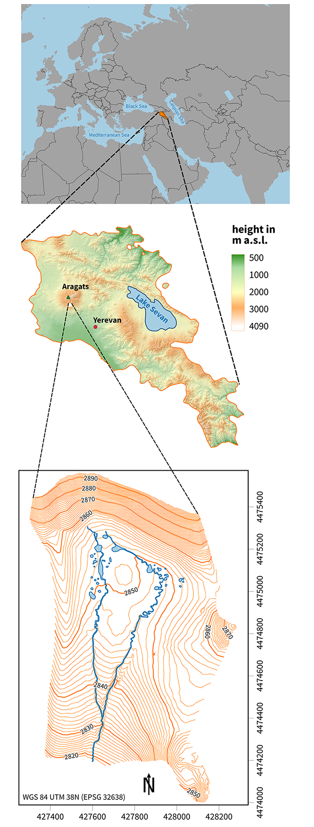
Figure 1 Location of the study area Karmir Sar on Mount Aragats, Armenia. Map: J. Elicker; data: Natural Earth, Alos DEM
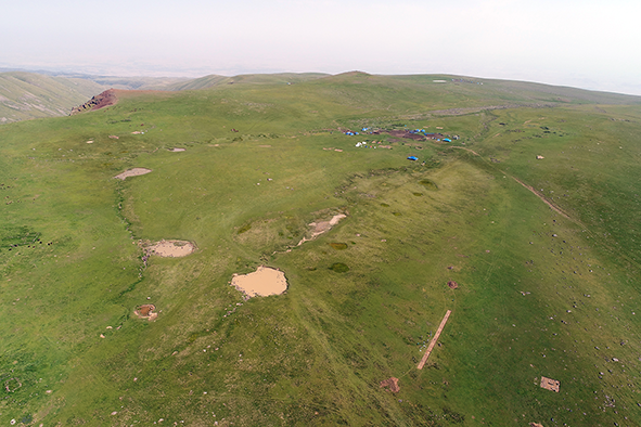
Figure 2 Karmir Sar. View of the central and lower part of the study area from the northwest. Photo: M. Rummel
2.1 Ground Control Points (GCP)
The excavation project on Karmir Sar uses 17 fixed points that are dispersed at different elevations over the site [fig. 3]. All points were measured in 2018 by Dr. Shahen Shahiniyan with a Leica GS10/15 GNSS rover receiver in static mode (30 minutes per point), combined with a Leica AR10/GR10 used as a reference station. Thanks to post-processing with base data (RINEX), the coordinates in WGS84/UTM 38N reference system were obtained with accuracy to the millimeter. The elevation values were converted from the ellipsoidal WGS84 height to the Baltic 1977 orthometric height using a proprietary quasi-geoid of Armenia (a previous version of this quasi-geoid is described in Margaryan 2014, the update by Shahinyan 2017 used in our case was not yet published). For purposes of this study, we rounded the elevation values to two decimal places.
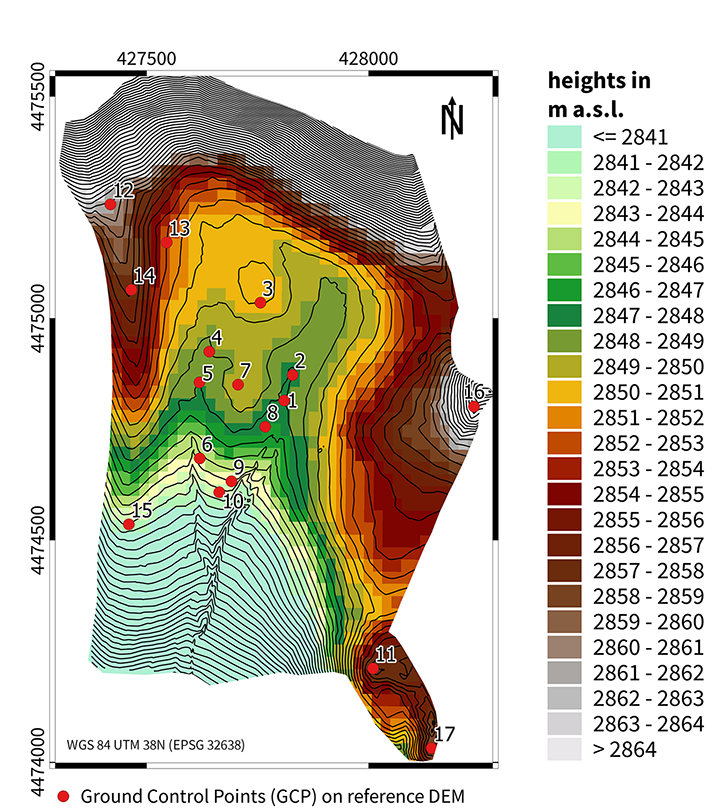
Figure 3 Position of high-definition ground control points at the study area. Map: J. Elicker
2.2 Reference DEM (RefDEM)
Previous research has demonstrated that a DEM derived from elevation contours of local topographic maps can be used as a reliable mean to reduce errors of global DEMs (Szypuła 2019). Our reference DEM, designated as RefDEM throughout this study, is derived from the contour plan of the archaeological site Karmir Sar. The contour plan, produced by geodesist Smbat Davtyan from Yerevan, has an interval of one meter between individual contour lines and covers an irregularly shaped area of circa 1.1 km2. Davtyan generated the contours in AutoCAD® software6 with standard settings of the create contour lines algorithm from 1735 points measured with a laser total station in 2012. Thanks to the presence of a geodetic triangulation point on site, it was possible to align the entire plan with the Armenian state grid. At the time of the plan’s completion in 2012, the coordinates were reported in the Gauss-Krüger Zone 8 coordinate system instead of Universal Transverse Mercator coordinate system used in Armenia today. The contour plan was originally georeferenced within the Pulkovo 1942 datum/Gauss-Krüger Zone 8 coordinate reference system (now deprecated) in order to obtain an overlap with local topographical maps of the entire Aragats area.
6 AutoCAD® 2007 Autodesk, Inc., https://www.autodesk.com/.
For the purposes of this study, the georeferenced vector contour plan was transformed into our RefDEM with a 25 m resolution. The conversion was conducted with the GRASS implement v.to.rast.attribute7 within the QGIS program8 (factor 25 set as raster size for adapting to the other DEMs in the best way possible). In this way, no data could be generated between the contour lines, so they were subsequently interpolated by the GRASS function r.surf.contour,9 which converted the previous patchy raster into a continuous DEM.
7 © 2003-2021 GRASS Development Team, GRASS GIS 7.6.2dev Reference Manual (Authors: Original code: Michael Shapiro, U.S. Army Construction Engineering Research Laboratory, GRASS 6.0 updates: Radim Blazek, ITC-irst, Trento, Italy, Stream directions: Jaro Hofierka and Helena Mitasova, GRASS 6.3 code cleanup and label support: Brad Douglas), https://grass.osgeo.org/grass78/manuals/v.to.rast.html.
8 All basic calculations and visualizations have been conducted within the program QGIS and its implemented functions, with the latest version at the given time: 2.18, 3.0 and 3.16 (QGIS.org, 2021. QGIS Geographic Information System. QGIS Association. http://www.qgis.org).
9 © 2003-2021 GRASS Development Team, GRASS GIS 7.6.2dev Reference Manual (Author: Chuck Ehlschlaeger, U.S. Army Construction Engineering Research Laboratory), https://grass.osgeo.org/grass78/manuals/r.surf.contour.html.
2.3 ALOS
The full name of this freely available DEM is ALOS Global Digital Surface Model (DSM) ‘ALOS World 3D-30m’, abbreviated in AW3D30.10 For our calculations, we have used its version 3.1 released in April 2020. ALOS is an acronym standing for Advanced Land Observing Satellite, nicknamed ‘Daichi’ and operated from 2006 to 2011 by the Japan Aerospace Exploration Agency. The ALOS elevation dataset was produced primarily from the processed stereo pairs of the PRISM (Panchromatic Remote-sensing Instrument for Stereo Mapping) optical instrument onboard the satellite (Tadono et al. 2016, 157-9). The spatial resolution of the originally developed 3D dataset is approximately 5 m, but the freely distributed DEM was reduced to a spatial resolution of approximately 30 m. In our study area, when using the projected WGS84/UTM38N coordinate reference system, one cell along the longitude corresponds to 21.2 m, along the latitude to 27.6 m.
The mask file (MSK extension) provided as a component of the ALOS dataset is a useful tool to retrace the origin of elevation values for each individual cell. It attests that the vast majority of cells in our study area was produced by the PRISM sensor of the ALOS satellite itself and their elevation was classified as valid (not distorted by snow or clouds). The few void cells concentrated on the slope in the northwest part of the study area were filled by using the SRTM1 V003 DEM [fig. 4]. The elevations in ALOS were converted from the ellipsoidal height, using the EGM96 geoid model (JAXA EORC 2020, 2).
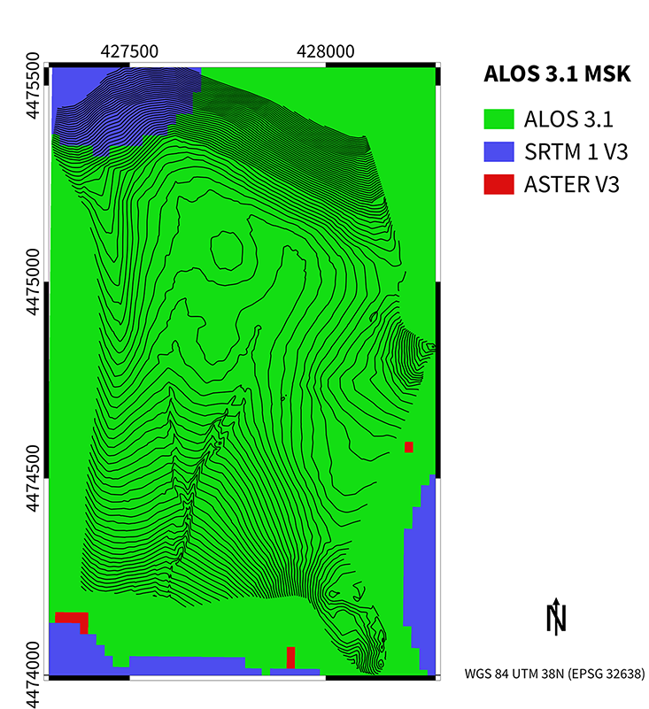
Figure 4 Void filled areas within the ALOS World 3D 3.1 version. Map: J. Elicker
2.4 ASTER
ASTER stands for Advanced Spaceborne Thermal Emission and Reflection Radiometer and it was released jointly by The Ministry of Economy, Trade, and Industry (METI) of Japan and the United States’ National Aeronautics and Space Administration (NASA).11 For our calculations we have used the Global Digital Elevation Model Version 3 (ASTER GDEM V3) released in August 2019. The original dataset was created photogrammetrically from a compilation of cloud-free ASTER stereopairs (DeWitt, Warner, Conley 2015, 182). ASTER GDEM V3 preferably used alternative DEMs to fill any voids before attempting to close them by an interpolation (Abrams, Crippen, Fujisada 2020, 5).
To identify the source of any given elevation cell value, the ASTER GDEM V3 dataset includes a numerical raster file (NUM extension). Its content indicates the number and the origin of scenes (stereo pairs) used to calculate the individual elevation values (Abrams et al. 2020, 7-8, table 3). In terms of internal assessment of quality, between ten to fifteen scenes are deemed sufficient; beyond that number the elevation error diminishes only marginally (Gesch et al. 2016, 145-6, fig. 5). According to the NUM file, our study area does not contain any voids filled with alternative DEMs; all cells were produced with stacking of 18 up to 30 ASTER GDEM V3 scenes and accordingly they not only fulfill, but also exceed the internal quality standards.
2.5 EU-DEM
The EU-DEM combines the advantages of both data acquisition techniques used for satellite remote sensing – the optical stereoscopy and radar interferometry.12 It is a blend of SRTM1 V003 and ASTER GDEM data, fused together by a weighted averaging approach and improved through Russian topographic maps, a hydrology dataset, proprietary high-precision elevation data and removal of artefacts (Bashfield, Keim 2011). It should be noted that its source data does not share the same level of detail – while the resolution of ASTER GDEM is 30 m, the SRTM3 dataset only has a resolution of ca. 90 m; the more precise SRTM1 dataset with 30m resolution was not freely available at the time for areas outside the United States of America. EU-DEM is provided with 25 m resolution, yet it is not specified in its documentation whether this improvement was achieved by simply upsampling the original lower-resolution datasets, or by enhancing them through proprietary high-precision data. For our analysis we have used the EU-DEM V1.1 version, released in 2016.
2.6 NEXTMap
The full name of this model, produced by the Intermap company, is NEXTMap World 30 DSM. Analogically to the EU-DEM, this model too is a fusion of other freely available datasets, specifically SRTM3 v2.1, ASTER GDEM v2.0, GTOPO30 (for polar areas). All datasets were void-filled, merged by a proprietary Intermap algorithm and their elevations were corrected with high-resolution LIDAR data from NASA’s Ice, Cloud and Land Elevation Satellite (Intermap 2013). The NEXTMap World 30DSM was marketed by Intermap as the “best-available surface elevation data with a 30-meter ground sampling distance” with a reliable and consistent global coverage (Intermap 2018). We have purchased the dataset for our area of interest in 2018, but in the meantime it was replaced by its successor with a higher, 10 m resolution.13 Though no versioning information has accompanied our dataset, we assume that it was NEXTMap World 30 DSM v2.0 released in 2013.14
14 Only two versions are publicized in the archive of Intermap press releases at https://www.intermap.com/pressreleases – the first version released in June 2012, the second in August 2013.
2.7 SRTM
In contrast to the ASTER and ALOS DEMs, which are based on optical stereoscopy, the SRTM (Shuttle Radar Topography Mission) DEM is based on the radar interferometry technique. The main advantage of the radar interferometry is that its data quality does not depend on light conditions. The interferometric synthetic aperture radar (InSAR) used by the mission has operated day and night, irrespective of the cloud cover (Rabus et al. 2003, 242). In fact, though the SRTM data covers nearly 80% of the earth’s land surface, they were collected within just 11 days – between 11th and 22nd February 2000 by the Endeavour shuttle (Farr, Kobrick 2000; Farr et al. 2007). For our analysis we have used SRTM1 Version 3 (also known as void-Filled SRTM Plus, SRTM NASA V3 or SRTMGL1 V003), which has a resolution of 1 arc-second (ca. 30 m) and had all of the previous voids filled.15 It was released in 2013 (NASA JPL 2013). The ancillary NUM file provided with this SRTM dataset attests that our study area had no voids filled with data from other sources. All its elevation values were classified as coming from either two or three SRTM swaths (for field coding cf. SRTM User Guide 2015).
2.8 NASADEM
NASADEM is a modernized version of the SRTM data. It was created by reprocessing the original raw SRTM signal data with improved algorithms, and by filling the voids with data from alternative sources (Buckley et al. 2020, 1, 5). For our analysis we have used the NASADEM Merged DEM Global 1 arc second Version 1 dataset, released in February 2020.16 Its resolution in our area is ca. 30 m. The ancillary NUM file provided with the NASADEM dataset attests that our study area had no voids filled with data from alternative sources. Its elevation values were classified as coming from SRTM radar swaths – the majority of cells from three swaths, with very few coming from just two swaths (for coding see Buckley et al. 2020, table 2).
3 Assessment Methodology
We have used three approaches to assess the quality of tested DEMs for geoarchaeological applications: a statistical comparison with ground control points, a statistical comparison with a reference DEM, and a visual assessment of the DEMs’ spatial structure (for a critical review of available assessment methods see Polidori, El Hage 2020). In this section we present the methods, the results are discussed in § 4.
3.1 Statistical Comparison with Ground Control Points
A common method of evaluating the quality of a DEM is to use a set of ground control points (GCP) measured precisely, and to compare their elevations with values at corresponding locations on the DEMs. By calculating the Root Mean Square Error (RMSE) of these values it is possible to statistically express the elevation discrepancies in meters between any tested model and the reference dataset. Comparing all tested models, the one with the lowermost RMSE value will have the least difference to the reference dataset and should thus be the one with the best vertical accuracy.
RMSE became a standard for determining the accuracy of maps (Ghilani 2017, 28) and it was frequently used by previous evaluations of DEMs (cf. e.g. Saran et al. 2010, 110; Nsanziyera et al. 2018). The advantage of the RMSE method is that, on one hand, the minus and plus errors will not neutralize themselves, but will all get treated equally. On the other hand, the outliers will have a substantial effect on the result because their weight will be exponentiated by the square function. The latter characteristic is a convenient method to differentiate between the quality of DEMs, where even a single substantial outlier can cause serious difficulties during various landscape analyses.
For our comparison, we have used the points described in § 2.1 as the reference dataset and computed the RMSE values (in meters) of all tested DEMs with the following equation:
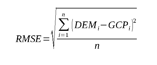
where i is the ground control point number, n is the total number of ground control points (in our case 17), GCPi is the elevation of the ground control point, DEMi is the elevation value of the cell corresponding to the position of the ground control point in the given DEM.
3.2 Statistical Comparison with the Reference DEM
While a statistical assessment with RMSE and GCPs offers a quick and precise glimpse on the vertical accuracy of DEMs, it is limited to a few cells that overlap with the position of GCPs, which can be misleading. One or few outliers can be concentrated on a limited area, on certain features, or on certain landscape types. The spatial distribution of errors thus plays an important role in recognizing error patterns and accordingly, whenever possible, it is meaningful to enhance the assessment of DEMs’ quality over their entire area. This can be achieved through comparisons with a reference DEM, which is usually less precise than ground control points, yet it offers the added benefit of being able to compare elevation cell values of the entire models.
In order to enable comparisons between the tested DEMs and the RefDEM, all available datasets needed to be adapted to matching parameters. We achieved this in two steps: in the first step, the RefDEM with a 25 m resolution was generated from the vector contour plan of the Karmir Sar site (see § 2.2) and in the second step, all raster images from the tested DEMs have been adjusted to the same size – to grant their correct overlay and correspondence of their cells. This was conducted within the raster calculator inside QGIS, where each model could be clipped to the exact same size as the RefDEM (rows: 47; columns: 57), resulting in matching position and size of all cells.17
17 Previous attempts to cut the models based on a polygon showed an imperfect overlay of raster cells. This can be attributed to differing projections of the underlying raw data, resulting in slight distortion of raster cells.
After adapting all datasets to matching parameters, the resulting clipped rasters were used to calculate the difference of height values of each cell with the raster calculator: values of each individually tested DEM were subtracted from values of the RefDEM. The outcome is either negative (RefDEM value is lower) or positive (RefDEM value is higher). For better visualization, each cell was then classified by means of a specific color – depending on the absolute difference in height. The height differences were divided up into one-meter steps, ranging between 9 and -9 m.
In addition, for the purpose of statistical evaluation, the values (height difference in meters) of each model´s cells have been extracted. This was achieved by creating sample points in the center of each cell with the raster pixels to points algorithm in QGIS. In order to avoid comparing distorted data from raster cells within the fringe range of the RefDEM, the outer sample points were deleted within a ‘buffer zone’ and not taken into consideration.18 Subsequently, the height difference values of each model´s cells have been extracted by the point sampling tool from the centered vector points (n=1569). These values were summarized within Excel and afterwards processed with JMP software19 to determine summary statistics (median, mean, minimum, maximum). Finally, the results were visualized as histograms to provide a closer examination of the value distribution.
18 A polygon surrounding the vector contour lines was created with the implemented tool concave hull (k-nearest neighbor).
19 Version JMP Statistics Pro 15 (SAS).
3.3 Visual Assessment of the Spatial Structure
For some applications, a surface consistency and a reliable rendering of terrain forms are more important than an absolute vertical accuracy, as long as an elevation offset is evenly distributed and not random. These characteristics are referred to as a “shape and topologic quality” (Polidori, El Hage 2020, 3) or also known as a “relative” or “geomorphological” accuracy (Szypuła 2019, 850). In order to assess them, the previous two statistic evaluations should thus be enhanced by a visual assessment of the spatial structure. An additional advantage of visual assessment is that it can also be done on each DEM intrinsically, without the need for external supplementary data. This is especially important for new field projects, where a convenient high-resolution reference dataset for comparisons rarely exists.
One of the easiest ways to gain a first impression of surface regularity, and even of the elevation difference regarding various models, is to make a cross-section. In our case, a cross section going from northwest to southeast was created for each model with the terrain profile tool of QGIS. After extracting the values (57 equally distributed points) along this selected line, they were visualized as line graphs within JMP Statistics. However, this approach only gives a first impression of the variation in terrain gradation for the selected models and, significantly, only in a restricted area.
A more comprehensive way to assess the spatial structure is to meaningfully visualize all elevation values. To ensure direct, cross-model visual comparison of elevation values and their distribution, all raster images need to be shown with standardized settings. For this purpose, the minimum and maximum values in the color style were adjusted to match the range of values at the location of Karmir Sar – with a minimum of 2840 m and a maximum of 2865 m a.s.l., following an elevation gain of one-meter steps. Simultaneously, the contour lines that served as a base for producing our RefDEM were put on top of each raster image to visualize the respective accordance in terrain gradation.
An additional approach regarding the assessment of elevation values distribution and surface regularity was to depict the models as shaded reliefs.20 Using this option, the quality of the data’s steadiness and possible errors by depicting or not depicting certain landscape features become even more distinguishable.
20 Implemented hillshade tool in QGIS (GDAL) with standard settings and a chosen z-factor of 0.00003.
4 Results and Discussion
All three assessment methods revealed considerable differences in the quality of the tested DEMs. However, it is interesting to note that the deployed assessment methods did not produce identical quality rankings, so a final combined assessment became necessary. We first present the results individually for each method, before proceeding to the combined assessment.
4.1 DEM Quality Assessment Based on Comparison with Ground Control Points
All tested DEMs, including the RefDEM generated from the contour plan, were compared with the GCP dataset using the methodology described in § 3.1 (for the description of datasets see §§ 2.1-2.8). The following Root Mean Square Errors (RMSE) have been calculated:
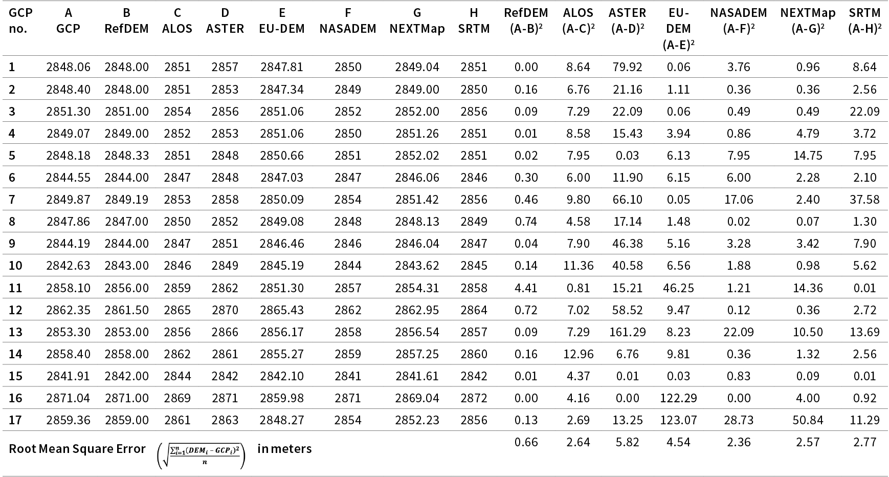 |
The comparison of the RMSE values demonstrates that our RefDEM has the lowest deviation from the high-precision GCP dataset. The deviation value of 0.66 m is a very good result, considering the creation of the RefDEM from a base contour plan with one-meter equidistance.21 It is a statistical confirmation of the fact that the RefDEM, which was produced from the most detailed dataset, comes closest to the high-precision control points and is accordingly the best suitable base for comparisons requiring entire surfaces.22
21 If it was not for a single outlier – the Ground Control Point no. 11 and its liminal position on the edge of a steep slope between two raster cells – the RMSE value would have been 0.50 m or better. This outlier is owed to the raster-creating algorithm that interpolated a medium value in the chosen 25 m cell size in a challenging terrain. Nonetheless, it is in the sense of the RMSE method to stress such deviations.
22 Since the GCP dataset is based on distinct and independent measuring methodology, the comparison with the RefDEM is legitimate and avoids circular reasoning.
The second-best result in terms of absolute vertical accuracy when compared with the GCP is held by the NASADEM dataset: 2.36 m. The RMSE values of ALOS, SRTM and NEXTMap came very close to each other; they range between 2.57 and 2.77 m. Considerably worse are the results for EU-DEM and ASTER, with values of 4.54 and 5.82 m, respectively. While the ASTER error is due to a number of randomly dispersed deviations in magnitude of 5 to 7 m and a single deviation in magnitude of almost 13 m, the substantial error of EU-DEM is caused by three points with 7 to 11 m deviation (GCPs no. 11, 16, 17), all of them close to the eastern limits of the contour plan. It looks as if the terrain modelled by EU-DEM near the three points was already sloping down towards the valley, though all the points are in reality located on the ridge. We suspect that this reflects either an intrinsic algorithm-based deformation of EU-DEM or a horizontal shift caused by the EU-DEMs projection.
4.2 DEM Quality Assessment Based on Statistical Comparison with the Reference DEM
Since its reliability and precision was confirmed by an assessment based on ground control points, the RefDEM can be considered a suitable base for visual and statistical comparisons with other DEMs where entire surfaces are required. For evaluating the whole extent of the study area, the deviation of height values from the RefDEM was calculated for each cell of every tested DEM raster (following the methodology described in § 3.2). The results were visualized in two ways: as a comparison of difference-rasters showing the spatial distribution of deviations [fig. 5], and as a histogram comparison of height differences in relation to cell count [fig. 6]. Both visualization types are interrelated and need to be mutually examined.
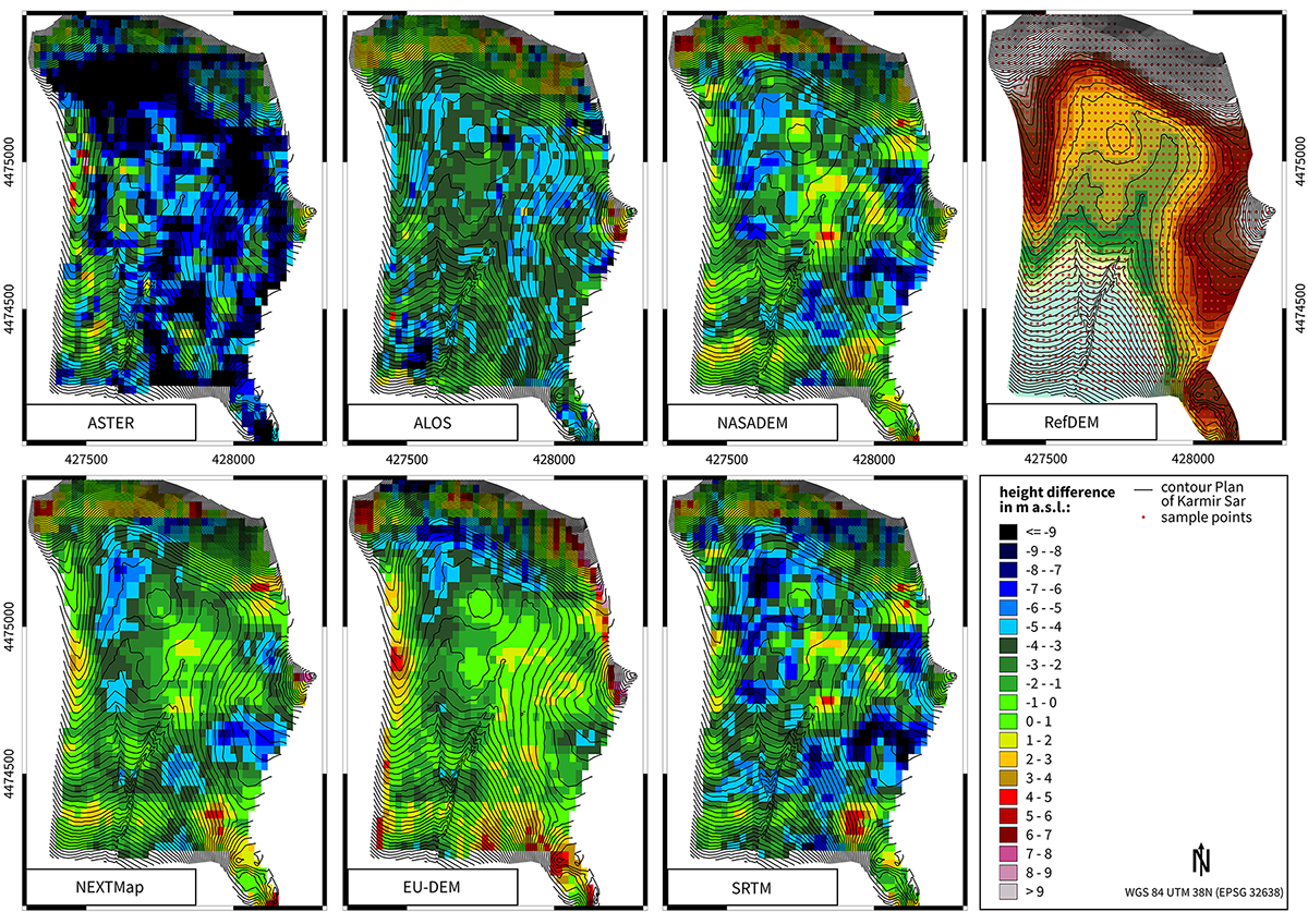
Figure 5 Distribution of differences in elevation between DEMs and the reference DEM with marked sample points within the cell centers. Map: J. Elicker
In general, both visualizations of height differences show that the majority of significant discrepancies lies within the negative range.23 This means the models in question depict higher elevation data than the original terrain. In particular, the spatial visualization of deviations allows several insights concerning the magnitudes of error and distribution of error clusters. The ASTER data evidently shows the largest area covered by highest deviations of -8 to <-9 m. In this range, the NASADEM and SRTM values differ more occasionally within smaller areas, which are irregularly distributed. The variation of these models rather lies within a lower range from -7 to -4 m. In both cases, significant leaps in value are noticeable. However, the NASADEM shows more spots ranging between 0 and -2 m of height difference than the SRTM data. The ALOS model depicts relatively widespread values between -1 to -4 m, while only limited areas show differences of -4 to -6 m or higher. The NEXTMap model as well as the EU-DEM show widespread variations to a lesser extent (mainly -2 to 2 m). Most of the higher difference values are still situated within a moderate scale and, in addition, more clustered in certain areas. Especially within the higher located areas in the north or east one can still find extreme variation up to -9 m, though they only appear in single spots.
23 It must be noted again that the areas outside the contour lines were ignored for they have no correctly interpolated values and consequently cannot reflect a reliable value in difference.
The second visualization enhances the first one by summarizing the statistical evaluation of height differences [fig. 6]. The histograms show the number of cells on the y-axis while depicting the difference of height in meters on the x-axis for each DEM. This way, one can perceive how many cells are situated within a certain range or increment of height difference (total number of included cells according to the marked sample points in fig. 5: N = 1569). Summary statistics such as minimum, maximum, mean and median are depicted on the right. Ideally, a DEM of favorable quality would be expected to show a low ranging spectrum, where the min. and max. values lie as close around 0 m of height difference as possible. Given a wider range, at least a clustering of values around 0 m would be expected, leaving only occasional cells within higher increments (negative or positive) so they can be determined as outliers. In both cases, the mean and median value should be close to 0 m and not differ significantly from each other.
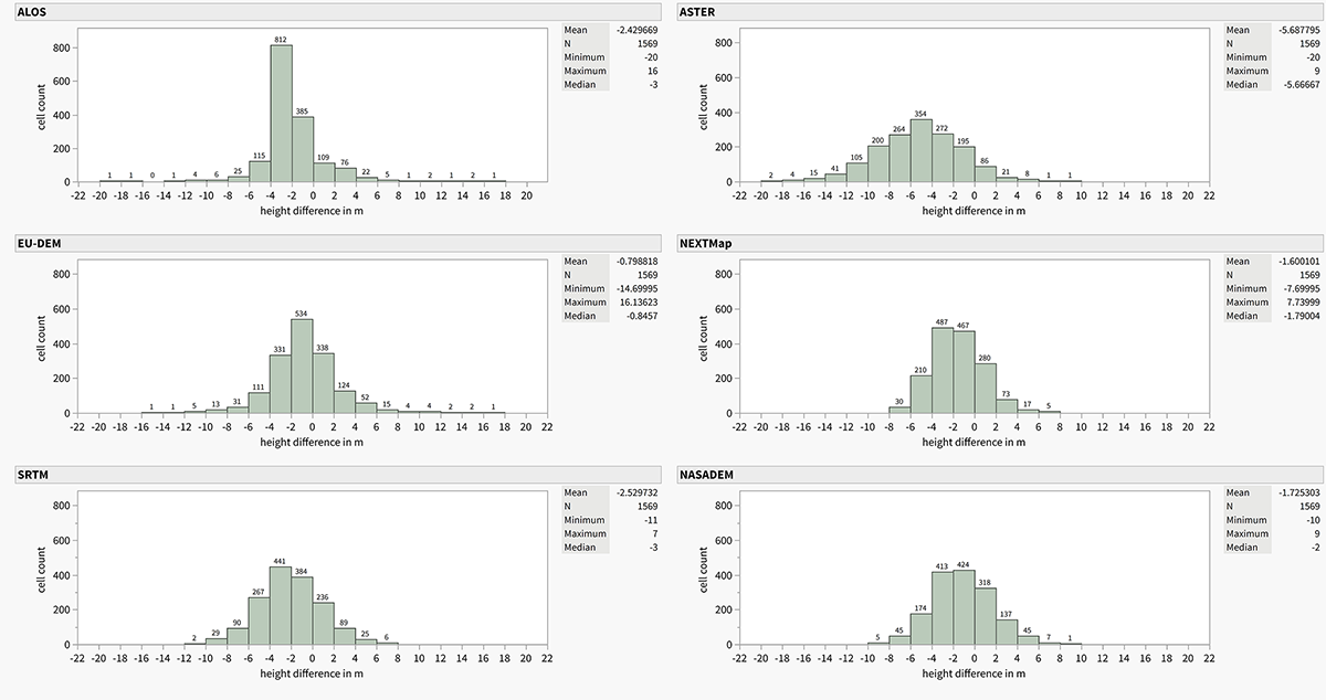
Figure 6 Distribution of differences in elevation according to cell count. Chart: J. Elicker
The ASTER data shows the most even distribution resulting in a flattened ‘curve’ with a vaguely distinguishable peak. The median and mean (-5.66 m and -5.68 m) are almost similar in value, but are also the ones furthest away from the ideal 0 m. The values’ range is slightly less scattered (min. -20 m; max. 9 m) than others, but the number of cells for each increment are more evenly distributed across the spectrum. Therefore, higher differences e.g. between -10 to -12 m still comprise about 105 cells.
The deviation range of the ALOS model (min. -20 m; max. 16 m) must be considered as extremely high. However, most values (812) have height differences ranging between -2 and -4 m, leaving a remarkable gap to neighboring increments. Higher increments (-6 to -20 m and 4 to 18 m) entail only a small share of cells in total. Those can be classified as outliers and do not heavily influence the overall impression of this model. The median (-3 m) and mean (-2.4 m) differ slightly, which is not ideal but an acceptable result, also regarding the values themselves.
While the mean (-1.7 m) and median (-2 m) of the NASADEM are slightly smaller and closer to each other compared to the ones of ALOS, a difference regarding the range is evident (min. -10 m; max. 9 m). Compared to its predecessor SRTM, a slight improvement is visible regarding both the range (min. -11 m; max. 7 m) as well as median (-3 m) and mean (-2.5 m). In both cases, the number of cells is rather clustered without many outliers, resulting in a less significant peak and, consequently, a higher and more evenly distributed share of cells within the increments. Nevertheless, the well rated range of NASADEM is only exceeded by NEXTMap (min. -7.7 m; max. 7.7 m), which reaches the best result in this regard. Also, in terms of median (-1.8 m) and mean (-1.6 m), the model comes out considerably well.
With a rather moderate range (min. -14.7 m; max. 16.1 m), the EU-DEM shows the best results regarding median (-0.85 m) and mean (-0.8 m). Even so, the highest increments in height difference only include minimal numbers of cells in total and can be classified as outliers. Therefore, the significant number is situated between -6 to 6 m and, including median and mean, this model shows the most favorable statistics.
4.3 Visual Assessment of DEMs’ Quality
For visual comparisons focusing mainly on terrain gradation, we used a visualization with multi-color elevation rendering and a hillshade visualization. In addition to these two separated comparisons between the RefDEM and the tested models, a cross section was used to depict the differences of all models simultaneously within a selected area (see § 3.3 for more details). Although all tested models were compared to the RefDEM, these three visualization methods convey important autonomous insights into model quality and would allow some primary assessment even without a reference dataset.
4.3.1 Visualization of Terrain Profiles with a Cross-Section
The cross section follows a northwest to southeast running line [fig. 7]. Its position was chosen with the aim of cutting through areas with the highest topographic variability. Thanks to this visualization, all tested DEMs can be compared in a single figure.
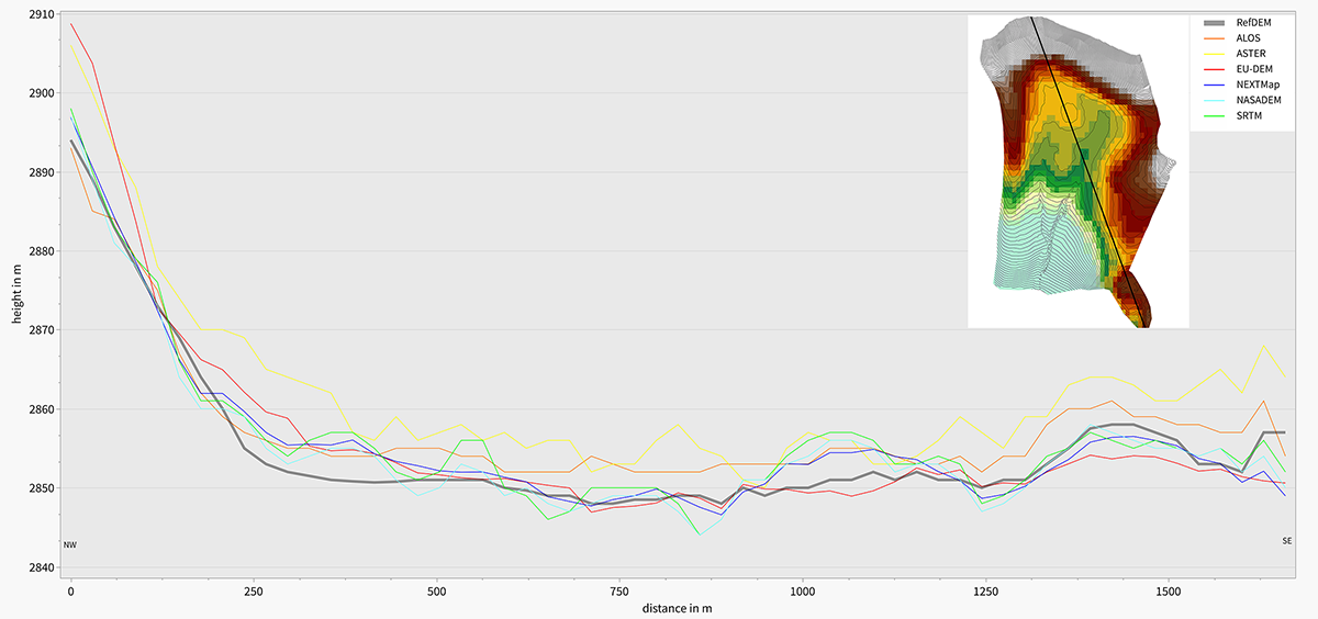
Figure 7 Differences of terrain gradation between the DEMs from a cross section going northwest to southeast. Chart: J. Elicker
In this cross-section the volatile and inconsistent character of NASADEM, SRTM and ASTER is evident, though the former two at least range in the vicinity of the RefDEM´s height level. For the most part, ASTER depicts by far the highest values throughout its whole course. At the same time, all other models show a little more steadiness. While the northwestern region (between 0 and 125 m in distance) is very closely resembled by ALOS, NEXTMap, NASADEM and SRTM, a significant difference of more than 10 m for the two remaining models is evident. Apart from this particular spot, EU-DEM generally follows the original landscape with differences of more than 5 m in certain areas. However, ALOS follows the original course most closely, but with a consistent gap of a few meters. Within the already above-mentioned plain area (between 250 to 625 m distance) the data suggests – besides complete irregularity in cases of ASTER, NASADEM and SRTM – higher elevations from 5 up to 15 m for all models.
4.3.2 Visualization of the Terrain with Multi-Color Elevation Rendering in Discrete 1-Meter Steps
Regarding the spatial visualization with multi-color elevation rendering in discrete 1-meter steps, some differences between the open data models are already obvious at first sight [fig. 8]. Especially the ASTER dataset seems to contain an extremely irregular and volatile distribution of values. No natural gradation whatsoever is recognizable, and a correlation with the RefDEM is scarcely apparent, with the exceptions of the higher regions within the north as well as the eastern peak. Nonetheless, values higher than 2861 m are extensively widespread, which does not correspond to reality. The NASADEM is of only slightly better quality in this regard and shows only small differences compared to SRTM. For both models, the values of the cells follow a smoother gradation, though they still contain some evident leaps. Nevertheless, the models only match the RefDEM in limited areas and those values themselves are mostly much higher than the original landscape. This is especially evident by looking at the plain in the middle of the northern half (originally at a height between 2850 - 2851 m a.s.l.) and, again, the eastern peak.
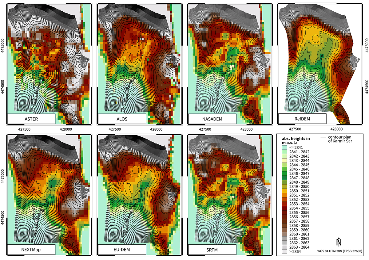
Figure 8 Spatial visualization of surface regularity for the different DEMs in Karmir Sar. Map: J. Elicker
Within the ALOS model, different topographic features are discernible e.g., the two north-south depressions are indicated, and irregularities as well as volatile transitions are shown only occasionally. The terrain is fairly coherent, particularly within the lower regions. Nevertheless, the whole area generally seems to be depicted as higher than the RefDEM suggests the original terrain to be.
By far the best quality of all compared open data models is shown by the EU-DEM. The terrain gradation is both clearly visible and smooth, without any sudden or extreme leaps. Topographic features are distinct and match the contour lines of the RefDEM more closely. Even the eastern depression is clearly indicated in its entire length. Only few differences remain in comparison to the natural terrain. For instance, the plain is less discernible and the western depression reaching from north to south is less pronounced than it should be.
The charged model NEXTMap World 30 is quite similar to the EU-DEM, e.g. it also appears to misrepresent the plain and the western depression. Only a few differences in quality between these two models can be pointed out. Especially, the accordance with the original terrain is exceeded by the EU-DEM in some areas (like the eastern depression). The general terrain gradation is comparable to the EU-DEM, but with slightly higher values in total. Even though the quality of both models seems to be comparably high, a small apparent difference to the RefDEM, and therefore to the original terrain, remains.
4.3.3 Visualization of the Models as Shaded Reliefs
Differences in terrain gradation become likewise visible when looking at the visualization of the models as shaded reliefs [fig. 9]. This hillshade view offers a more detailed impression regarding gradation and continuity of the data. The volatile and unsteady character of the ASTER, NASADEM and SRTM data stands out, while the remaining ones occasionally show landscape features, which do not – or at least not to the depicted extent – exist in reality: e.g. the distinctive mound in the middle of the northern area (ALOS), or the extended spaciousness of the easternmost peak (EU-DEM and NEXTMap). Nevertheless, apart from the RefDEM, ALOS as well as EU-DEM show the closest resemblance by depicting a generally flat and smoothly undulating landscape. In this regard, the NEXTMap model depicts a more irregular terrain than the previous visualization suggested. EU-DEM shows some jittery effects that might be caused by algorithm smoothing or reprojection issues.
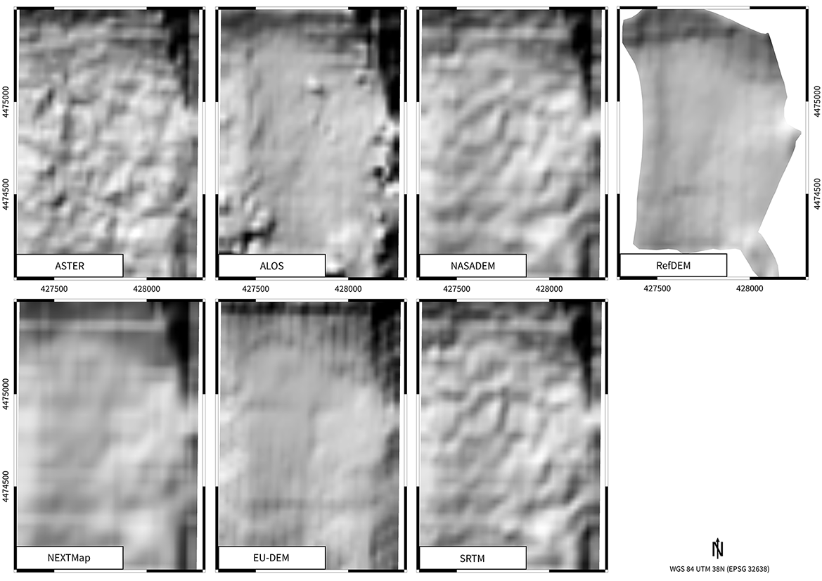
Figure 9 DEMs depicted as shaded reliefs as an additional approach to examine surface continuity and point out irregularities. Map: J. Elicker
4.4 Combined Assessment
As already indicated in the introduction to this section, and corroborated in its previous subsections, the various assessment methods led to some differences in rankings. The assessment with GCP placed NASADEM as the most accurate, followed by NEXTMap and ALOS. According to the assessment with RefDEM the first place belongs to EU-DEM, followed by NEXTMap and NASADEM. Finally, the visual assessments revealed the following sequence: EU-DEM first, NEXTMap second, and ALOS third. What all rankings have in common is the last position achieved by the ASTER model.
But which ranking is then most useful and which model can be recommended as the best? Evidently, each assessment method has its advantages and limitations. The advantage of the assessment with GCP lies in its high precision, yet it is limited by a reduced comparison area. The assessment with a reference DEM uses complete areas for comparisons, yet it has lower precision and is not sufficient for detecting surface flaws. The visual assessment does detect surface flaws, yet it does not quantify them. So, in order to understand which DEMs do best represent a landscape, it is useful to combine the advantages of all assessment methods. At the end, the result also depends on the intended use of the models.
In consequence, the ASTER, NASADEM, and to a much lesser degree also ALOS, demonstrate modelled surfaces that are uneven, distorted and contain artifacts. This overrides some statistically good results and limits the use of these models for geoarchaeological purposes. In case of viewshed analyses, the randomness and the magnitude of such irregularities effectively hinders the use of affected DEMs as a reliable source. A similar conclusion applies for hydrological applications, unless intended in a low resolution. Regarding the NASADEM and SRTM, which are based on the same data, the more recent NASADEM indeed obtained better results in every assessment method for our study area. It is to be expected that NASADEM is going to replace SRTM in the near future.
For our studies on the open treeless subalpine landscape of Mount Aragats, the combined assessment reveals that among all tested DEMs the most suitable ones are the EU-DEM and NEXTMap. They are both very similar in quality, and were produced with nearly identical methodology, involving the proprietary algorithms of the Intergraph company (also by EU-DEM, cf. Bashfield, Keim 2011). Both EU-DEM and NEXTMap 30 DSM are largely free of artifacts and are consequently more reliable and consistent, probably as a result of smoothing algorithms, fusing with a lower resolution SRTM3 dataset (90 m), and the removal of spikes. NEXTMap has markedly better mean elevation precision, while EU-DEM is slightly better in modelling the terrain shapes. The main advantage of NEXTMap is its global coverage, while the main advantage of EU-DEM is its availability at no cost.
4.5 Interpretations and Limitations
Our study area in high mountains is topographically very static, so the temporal aspect of data collection does not play a crucial role. However, there are two relevant, seasonally recurring patterns to consider as exceptions. First, every winter season the study area is covered by several meters of snow, so any data acquired remotely in this period can be expected to be systematically higher than the actual terrain. Second, seasonal pastoralists traditionally visit the study area during the summer months, and they build their large tents in the middle of it. Depending on the time of the data collection, there could theoretically be differences of up to three or four meters in the limited central area of the site where the tents temporarily stood.
The first recurring pattern could explain the thoroughly higher elevations in case of SRTM as well as NASADEM, and to a certain degree also EU-DEM and NEXTMap. All four models are based on (or incorporate) data from the SRTM mission, which was collected in February 2000, when our high-altitude study area was in the peak of the winter season and must have been covered by several meters of snow. To a certain degree, the presence of snow might be responsible for the higher elevations of ALOS and ASTER, too. Though both latter models were produced by stacking of image pairs acquired over several years, their elevations resulted from averaging all values, presumably including the extreme winter ones. Snow surfaces are notoriously difficult to model with optical photogrammetry due to point alignment issues on homogeneous backgrounds.
Concerning the second recurring pattern, we examined the option that some of the irregularities in ASTER and ALOS might have been caused by seasonal pastoralist activities. However, we concluded that this is not necessarily the case, as the irregularities in the models do not concentrate exclusively on the central area, which is being recurrently used by the pastoralists. The irregularities thus must have been caused by other conditions.
What might these conditions have been? Irregularities in form of spikes are typical for models based on optical stereoscopy and are likely caused by point mismatches in the image pairs; they occur locally as jumps between two adjacent pixels (Honickel 1999; Karkee, Steward, Aziz 2008, 294). A number of similar errors like ‘bumps’, ‘pits’, ‘mole-runs’, other geometric artifacts, and grainy anomalies (‘noise’) have been reported for previous versions of ASTER, especially for areas with insufficient image coverage, persistent clouds or suspected abundant snow cover (ASTER GDEM Validation Team 2009, 22-6; 2011, 18). Yet, irregular artifacts evidently persist even in the newest, third ASTER version and in spite of sufficient imagery coverage (see §§ 2.4 and 4.3). We can only speculate about the reasons – insufficient light conditions, differences between periods with and without snow cover, reflection from the water surface of the small ponds, and missing contrast in times with snow cover are among the most likely options.
Radar interferometry avoids some of the errors typical for optical stereoscopy (cloud errors, snow and water reflection errors, insufficient light contrast), yet this technique is susceptible to other errors, some of which also produce geometric artefacts or voids (failings under high terrain steepness or rapid change in surface roughness, specular reflection errors of water areas, deserts and other surfaces that reflect too little microwave energy, radar shadows, radar correlation and phase-unwrapping errors).24 This seems to be confirmed in our case, where the visualizations of SRTM and NASADEM also displayed various artifacts.
24 Rodríguez, Morris, Belz 2006; Karkee, Steward, Aziz 2008, 294; Yang, Meng, Zhang 2011.
At last, an additional option to explain the generally higher elevations of all DEMs based on satellite remote sensing methods in our study area should be discussed. It is a possible systematic offset caused by using different geoids for transformation between the ellipsoidal and the orthometric heights. Our ground control points were transformed using the proprietary high-precision quasi-geoid of Armenia, which yields values nearly identical to the heights used in local topographic maps and to our RefDEM. The satellite models, on the other hand, were transformed with either EGM96 (Earth gravitational model from 1996 used for ALOS, ASTER, NEXTMap, NASADEM, SRTM) or EGG08 (European gravimetric geoid/quasi-geoid from 2008 used for EU-DEM). A quick test for a trigonometric geodetic point in Tirinkatar (= our GCP no. 17 with an ellipsoidal height = 2883.939 m) revealed that its height recorded in the Armenian cadaster office is 2859.20 m, in topographic maps it is 2859.10 m;25 transformed with the quasi-geoid of Armenia it is 2859.36 m, while transformed with EGM96 it is 2861.03.26 We could not find out the exact transformation value with EGG08, but a transformation with similar EGM2008 (Earth Gravitational Model from 2008, recommended for areas outside continental Europe) yielded an elevation value of 2860.02 m.27 This implies that if all elevation datasets were transformed to the same vertical reference system, the observed difference between the height values of our tested DEMs and the RefDEM could be lowered by up to 2 m, thus making most datasets derived from satellite data comparable to the RefDEM in terms of absolute elevations (see table 1). We did not execute these transformations because we were interested in assessing the quality of DEMs in the form in which they are distributed. However, if the expected improvement in accuracy were confirmed, it would be a remarkable result, partly improving the impression that the vertical accuracy of the freely available global DEMs is their grave limitation (Schumann, Bates 2018).
25 Soviet military map K-38-125-V in 1:50 000 scale from 1974.
26 Calculated online at https://geographiclib.sourceforge.io/cgi-bin/GeoidEval.
27 Recommendation from INSPIRE 2013: VI, 75. The value calculated online at https://geographiclib.sourceforge.io/cgi-bin/GeoidEval.
5 Conclusions
Regarding the first objective formulated in the introduction section – to understand why ASTER failed to provide convincing results in the first landscape study (Anselm 2012) – we have reached the following conclusion. The visual assessment provided evidence that ASTER’s modelled surface of our study area is covered by abrupt and random spikes between neighboring cells of up to 10 m in magnitude. We identify these spikes as the cause of misleading results encountered during the visibility analysis of prehistoric stone steles in Karmir Sar. Any higher spike occurring between two steles, or even a lower spike positioned close to the observer or the observed point, inevitably interrupts the computed line of sight and the visibility analysis returns a negative result. Since the spikes do not exist in the real world, they distort the digital elevation model and falsify analyses based on it.
Regarding our second objective – to find out whether other available DEMs based on satellite remote sensing data did represent the local topography more appropriately – we report a positive result. According to all our assessment classifications, the ASTER DEM finished with the worst scores in our study area and all other tested DEMs did better, some of them considerably. The best result in terms of vertical accuracy was assessed by the NASADEM (RMSE of 2.36 m against 5.82 m in case of ASTER), yet NASADEM also suffers, though to a smaller extent than ASTER, from random spikes. When considering the surface regularity and accuracy, the best results were obtained for EU-DEM and NEXTMap, whose surfaces were algorithmically smoothed and, as a consequence, are more reliable.28
28 E.g., the visibility analysis of the steles leads in case of using NEXTMap to 18, in case of EU-DEM to 24, in case of refDEM to 26 positive results out of 30 possible combinations (in contrast to 3 positive results in case of ASTER, cf. Introduction).
To conclude, we would like to express a warning and a recommendation. A warning against the uncritical use of our (and any other) results for choosing the best available DEM, even in study areas with supposedly comparable landscape and vegetation characteristics. Instead, we strongly recommend assessing the suitability of available DEMs for every study area separately, with an assessment strategy calibrated for the needs of the intended analysis. This may sound self-evident, but it is rarely done for archaeological projects. In the absence of precise reference datasets against which the DEMs could be checked, we recommend choosing a small area (1-2 km2), zooming in to distinctly visualize all of its pixels and then visually assessing whether it corresponds with the expectations (see § 3.3). Preferably, it should be an area that can be compared to one’s own empirical experience, or – if the evaluator has no prior first-hand knowledge of the landscape – some area known to be largely even or flat.
Abbreviation list
|
ALOS |
ALOS World 3D 30 m 3.1 |
|
a.s.l. |
above sea level |
|
ASTER |
ASTER GDEM V3 |
|
DEM |
Digital Elevation Model |
|
DSM |
Digital Surface Model |
|
DTM |
Digital Terrain Model |
|
EU-DEM |
EU-DEM V 1.1 |
|
EGM96 |
Earth Gravitational Model |
|
GCP |
Ground Control Points |
|
LIDAR |
Light Detection and Ranging |
|
MSK |
mask file extension for ALOS |
|
NASADEM |
NASA Merged DEM Global 1 arc second Version 1 |
|
NEXTMap |
NEXTMap World 30 DSM |
|
RefDEM |
Reference DEM derived from high precision points for Karmir Sar |
|
RINEX |
Receiver Independent Exchange Format |
|
RMSE |
Root Mean Square Error |
|
SRTM |
Shuttle Radar Topography Mission 1 V003 |
|
WGS |
World Geodetic System |
Bibliography
Abrams, M.; Crippen, R.; Fujisada, H. (2020). “ASTER Global Digital Elevation Model (GDEM) and ASTER Global Water Body Dataset (ASTWBD)”. Remote Sensing, 12(7), 1156. https://doi.org/10.3390/rs12071156.
Anselm, N. (2012). GIS-unterstützte Sichtbarkeitsanalyse von Drachensteinen im Armenischen Hochland [BA Thesis]. Freie Universität, Fachbereich Geowissenschaften, Institut für Geographische Wissenschaften, Physische Geographie, Berlin.
ASTER GDEM Validation Team (2009). ASTER Global DEM Validation. Summary Report. p. 28. https://lpdaac.usgs.gov/documents/28/ASTER_GDEM_Validation_1_Summary_Report.pdf.
ASTER GDEM Validation Team (2011). ASTER Global Digital Elevation Model Version 2 - Summary of Validation Results. p. 27. https://ssl.jspacesystems.or.jp/ersdac/GDEM/ver2Validation/Summary_GDEM2_validation_report_final.pdf.
Bashfield, A.; Keim, A. (2011). “Continent-wide DEM Creation for the European Union”. 34th International Symposium on Remote Sensing of Environment. The GEOSS Era: Towards Operational Environmental Monitoring (Sydney, 10-15 April 2011). https://www.isprs.org/proceedings/2011/ISRSE-34/.
Bongers, J.; Arkush, E.; Harrower, M. (2012). “Landscapes of Death: GIS-Based Analyses of Chullpas in the Western Lake Titicaca Basin”. Journal of Archaeological Science, 39(6), 1687-93. https://doi.org/10.1016/j.jas.2011.11.018.
Buckley, S.M. et al. (2020). NASADEM (User Guide). Pasadena: National Aeronautics and Space Administration, Jet Propulsion Laboratory, California Institute of Technology, 48. https://lpdaac.usgs.gov/documents/592/NASADEM_User_Guide_V1.pdf.
Conolly, J.; Lake, M. (2006). Geographical Information Systems in Archaeology (Illustrated edition). Cambridge: Cambridge University Press.
DeWitt, J.D.; Warner, T.A.; Conley, J.F. (2015). “Comparison of DEMS derived from USGS DLG, SRTM, a Statewide Photogrammetry Program, ASTER GDEM and LiDAR: Implications for Change Detection”. GIScience & Remote Sensing, 52(2), 179-97. https://doi.org/10.1080/15481603.2015.1019708.
Dungan, K. et al. (2018). “A Total Viewshed Approach to Local Visibility in the Chaco World”. Antiquity, 92(364), 905-21. https://doi.org/10.15184/aqy.2018.135.
Farr, T.G.; Kobrick, M. (2000). “Shuttle Radar Topography Mission Produces a Wealth of Data”. Eos, Transactions American Geophysical Union, 81(48), 583-5. https://doi.org/10.1029/EO081i048p00583.
Farr, T.G. et al. (2007). “The Shuttle Radar Topography Mission”. Reviews of Geophysics, 45(2). https://doi.org/10.1029/2005RG000183.
Gesch, D.B. et al. (2016). “Validation of the ASTER Global Digital Elevation Model Version 3 Over the Conterminous United States”. XXIII ISPRS Congress (Prague, 12-19 July 2016). The International Archives of the Photogrammetry, Remote Sensing and Spatial Information Sciences, XLI-B4, 143-8. https://doi.org/10.5194/isprs-archives-XLI-B4-143-2016.
Ghilani, C.D. (2017). Adjustment Computations: Spatial Data Analysis. 6th ed. Hoboken: John Wiley & Sons.
Gillings, M.; Hacıgüzeller, P.; Lock, G. (eds) (2020). Archaeological Spatial Analysis: A Methodological Guide. London: Routledge. https://doi.org/10.4324/9781351243858
Hirt, C. (2014). “Digital Terrain Models”. Encyclopedia of Geodesy, 1-6. https://doi.org/10.1007/978-3-319-02370-0_31-1.
Honikel, M. (1999). “Strategies and Methods for the Fusion of Digital Elevation Models from Optical and SAR Data”. International archives of photogrammetry and remote sensing (ISPRS), 32(7-4-3W6), 83-9.
INSPIRE (2013). D2.8.II.1 INSPIRE Data Specification on Elevation–Technical Guidelines. European Commission Joint Research Centre, Thematic Working Group Elevation, 200. https://inspire.ec.europa.eu/file/1530/download?token=pq85sbLG.
Intermap (2013). Technical Review. NEXTMap® World 30TM Digital Surface Model (Technical Review No. 083013v3). Englewood: Intermap Technologies, 12.
Intermap (2018). NEXTMap® World 30TM Data Sheet. https://www.intermap.com/hubfs/NEXTMap_World30_Data-Sheet.pdf.
JAXA EORC (2020). ALOS Global Digital Surface Model (DSM). ALOS World 3D-30m (AW3D30). Version 3.1 (Product Description). Earth Observation Research Center, Japan Aerospace Exploration Agency (JAXA EORC). https://www.eorc.jaxa.jp/ALOS/en/aw3d30/aw3d30v31_product_e_a.pdf.
Karkee, M.; Steward, B.L.; Aziz, S.A. (2008). “Improving Quality of Public Domain Digital Elevation Models Through Data Fusion”. Biosystems Engineering, 101(3), 293-305. https://doi.org/10.1016/j.biosystemseng.2008.09.010.
Lambers, K.; Sauerbier, M. (2007). “A Fresh View on the Nasca Lines: Investigating Geoglyph Visibility in Palpa (lca, Peru)”. Clark, J.T.; Hagemeister, E. (eds), Digital Discovery: Exploring New Frontiers in Human Heritage; Proceedings of the 34th Conference on Computer Applications and Quantitative Methods in Archaeology (Fargo, 18-22 April 2006). Budapest: Archaeolingua, 228-38.
Margaryan, V. (2014). “Analysis of Quasi-Geoid Model Created for Territory of the Republic of Armenia”. Advanced Materials Research, 1020, 484-7. https://doi.org/10.4028/www.scientific.net/AMR.1020.484.
Marsh, E.J.; Schreiber, K. (2015). “Eyes of the Empire: A Viewshed-Based Exploration of Wari Site-placement Decisions in the Sondondo Valley, Peru”. Journal of Archaeological Science: Reports, 4, 54-64. https://doi.org/10.1016/j.jasrep.2015.08.031.
NASA JPL (2013). NASA Shuttle Radar Topography Mission Global 1 arc second [data set]. NASA EOSDIS Land Processes DAAC. https://doi.org/10.5067/MEASURES/SRTM/SRTMGL1N.003.
Nsanziyera, A.F. et al. (2018). “Remote-Sensing Data-Based Archaeological Predictive Model (APM) for Archaeological Site Mapping in Desert Area, South Morocco”. Comptes Rendus Geoscience, 350(6), 319-30. https://doi.org/10.1016/j.crte.2018.06.010.
Polidori, L.; El Hage, M. (2020). “Digital Elevation Model Quality Assessment Methods: A Critical Review”. Remote Sensing, 12(21), 3522. https://doi.org/10.3390/rs12213522.
Rabus, B. et al. (2003). “The Shuttle Radar Topography Mission—A New Class of Digital Elevation Models Acquired by Spaceborne Radar”. ISPRS Journal of Photogrammetry and Remote Sensing, 57(4), 241-62. https://doi.org/10.1016/S0924-2716(02)00124-7.
Rodríguez, E.; Morris, C.S.; Belz, J.E. (2006). “A Global Assessment of the SRTM Performance”. Photogrammetric Engineering & Remote Sensing, 72(3), 249-60. https://doi.org/10.14358/PERS.72.3.249.
Saran, S. et al. (2010). “Evaluation of Digital Elevation Models for Delineation of Hydrological Response Units in a Himalayan Watershed”. Geocarto International, 25(2), 105-22. https://doi.org/10.1080/10106040903051967.
Schumann, G.J.-P.; Bates, P.D. (2018). “The Need for a High-Accuracy, Open-Access Global DEM”. Frontiers in Earth Science, 6, 225. https://doi.org/10.3389/feart.2018.00225.
Shahinyan, S.Z. (2017). The Update of Quasi-Geoid Model of the Republic of Armenia and the Efficiency of Its Usage in the Field of Geodesy and Cartography [PhD Dissertation] (in Armenian language). Yerevan State University of Architecture and Construction. http://etd.asj-oa.am/6768/.
Siart, C.; Forbriger, M.; Bubenzer, O. (eds) (2018). Digital Geoarchaeology: New Techniques for Interdisciplinary Human-Environmental Research. Cham: Springer. https://doi.org/10.1007/978-3-319-25316-9.
SRTM User Guide (2015). The Shuttle Radar Topography Mission (SRTM) Collection User Guide. https://lpdaac.usgs.gov/documents/179/SRTM_User_Guide_V3.pdf.
Szypuła, B. (2019). “Quality Assessment of DEM Derived from Topographic Maps for Geomorphometric Purposes.” Open Geosciences, 11(1), 843-65. https://doi.org/10.1515/geo-2019-0066
Tadono, T. et al. (2016). “Generation of the 30 m-Mesh Global Digital Surface Model by Alos Prism”. XXIII ISPRS Congress (Prague, 12-19 July 2016). The International Archives of the Photogrammetry, Remote Sensing and Spatial Information Sciences, XLI-B4, 157-62. https://doi.org/10.5194/isprs-archives-XLI-B4-157-2016.
Triplett, E. (2016). “Visualizing Medieval Iberia’s Contested Space Through Multiple Scales of Visibility Analysis”. Forte, M.; Campana, S. (eds), Digital Methods and Remote Sensing in Archaeology: Archaeology in the Age of Sensing. Cham: Springer, 199-227. https://doi.org/10.1007/978-3-319-40658-9_9.
Yang, L.; Meng, X.; Zhang, X. (2011). “SRTM DEM and its Application Advances”. International Journal of Remote Sensing, 32(14), 3875-96. https://doi.org/10.1080/01431161003786016.
Zhou, Q. (2017). “Digital Elevation Model and Digital Surface Model”. Richardson, D.; Castree, N.; Goodchild, M.F.; Kobayashi, A.; Liu, W.; Marston, R.A. (eds), International Encyclopedia of Geography: People, the Earth, Environment, and Technology. John Wiley & Sons, 1-17. https://doi.org/10.1002/9781118786352.wbieg0768.